Last week the United Nations released estimates for global population (PDF alert) for the year 2100. In the low growth case it is expected to reach over 8 billion souls by 2050 before declining to some 6 billion by 2100; in the high growth case they anticipate a population of some 15 billion; with a median case of 10 billion people in 2100. That's a lot of people; given current resource demands and stresses on the environment today, it gets one thinking about steady state economies, how they might work, what the term even means. And when one thinks of steady state economies one naturally thinks of

And when one thinks of bunnies, one's mind inevitably turns to ...
Math.
On bunnies
If one is a boy bunny and the other a girl bunny then it is quite likely that we'll soon get more bunnies. And if we have more bunnies, we'll get even more bunnies, and so on and so forth. We can depict that graphically:
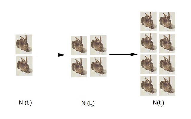
Evidently our population N increases at a rate proportional to the actual bunny population, which we can write as
dN/dt = r N
where the time derivative is just the rate of change in our population N and our constant of proportionality r is the rate of growth. This is a mathematical model for our bunny population.
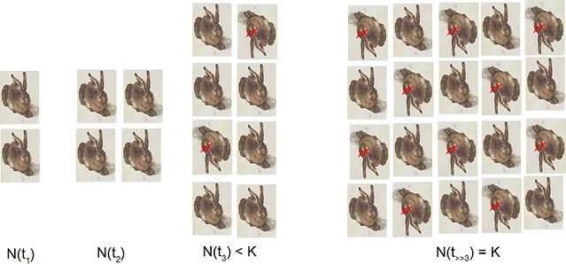
There's a problem with the model, of course: it's unbounded. In very little time we find ourselves drowning in bunnies. The good news is that there is a simple solution, the bad news is that the solution is exceedingly grim: our Bunnies Must Die. It doesn't much matter how -- predation, starvation, disease, bunny wars, peaceful senescence en route to the Great Carrot Patch in the Sky. The important thing is that there be a bound to the population.
Mathematically, we posit some maximum population (or carrying capacity) K such that N can never be greater than K, perhaps like this:
dN/dt = r N (K-N) / K
Exploring the limits we see that for small N, K-N ~= K, so (K-N) / K -> 1 and dN/dt ~= r N. For small populations N, the growth rate looks like our original model. At the other extreme, as the actual population N approaches the carrying capacity K, K-N -> 0, and the rate of population change dN/dt -> 0. Note that that's the rate of population change, not the population itself, which at that limit is approaching K. For the visually minded:
That equation above is known as the logistic equation or Verhulst equation, although you will likely see it in a slightly different form:
dx/dt = r x (1-x)
Here x = N/K, we rewrite the equation so that we are independent of the actual value of K: we've normalized the population range to go from zero (N = 0) to 1 (N = K). Integration is straightforward and plotting the results gives us (taken from the mathworld link)
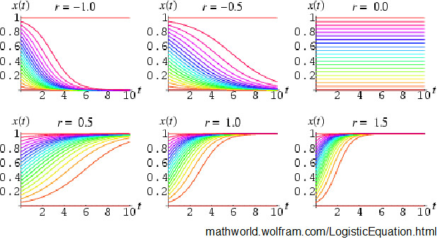
The colored lines are the trajectories (behavior in time) of various populations as color coded by initial population size, so the green lines are for an initial condition of x = 0.4 or so, blue for x = 0.6 or so, etc. Negative growth rates mean that death > birth and the population eventually dies out. When r = 0, there is neither net growth nor death and the populations are fixed at the initial conditions. Important to note is that as the magnitude of r increases, the rate at which the population reaches the final population (either 0 or 1, depending on the sign of r) increases. For large r, the population reaches the final population more quickly than at small r.
Our model is bounded and now well behaved. But, of course, we can always find ways of improving a model. In our case, because of things like seasons and the difficulty of finding things to eat in winter, bunny births are frequently timed so that the critters have a chance of surviving their first winter. That is, the population changes in a more stepwise rather than a continuous fashion. Really instead of a continuous derivative we need to discretize the steps. If we do so, our population size now depends on the population size of the step previous, perhaps like this:
x(t) = r x(t-1)(1 - x(t-1))
Here x(t) is our population N/K at time step t, x(t-1) is x at time step (t-1), etc. This is no longer a differential equation but a difference equation, specifically the logistic difference equation. A small change from the original, but in this case, discretization changes absolutely everything.
On attractors
Let's take a look at the behavior of the discretized equation.
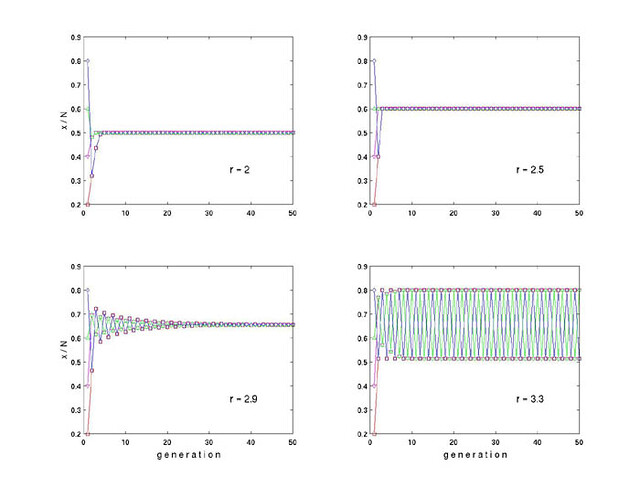
Here the horizontal axis (the "abscissa") is the number of generations, or time steps; the ordinate is the normalized population N/K (I see I switched terminology on you, on the plot it's labelled x/N, where x = N, N = K, x/N = oh never mind, you get the idea). Once again, the various lines are the trajectories for differing initial conditions.
Not obvious is that there are limits to r: for r < 1 the population is not stable and dies off, just like for negative r in the continuous case. For r > 4 or for x > 1 the solutions are not bounded: the population blows up (or down, can go to positive or negative infinity). But in the range of 1 <= r <= 4 there are a number of things to note.
First is that for 1 < r < 3 the trajectories converge to a population that is smaller than the carrying capacity K. If your initial condition N is greater than that stable population, you get a rapid die-off before reaching stabilization; if less, you get growth to the stable population. This is not the case for the continuous form of the logistic equation. As r increases, that final population increases. It also takes longer (more generations) to reach the stable population, and you get increasing "ringing" in the population as it settles to the final value. For r = 2.5, the population has stabilized within 5 generations, for r = 2.9 it is still settling down after 30 generations. These stable populations, btw, are mathematically known as fixed or stable attractors, because they are fixed values ("points in phase space", for the geek crowd) to which all trajectories converge, irrespective of initial condition.
Second thing to note: the stable population increases with r. That is, the attractors are r-dependent, which again is different from the continuous case. But then things get a bit strange: at r = 3 the system bifurcates: the ringing that is evident as r increases never settles down, so that solutions alternate between two stable populations. Not by much at first, but increasingly so with increasing r. By r = 3.3 those populations are at x ~0.5 and x ~0.8.
If we keep increasing r things get even stranger:
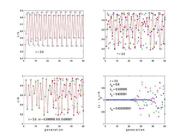
At r = 3.5 (top left) the system has bifurcated again and now 4 periodic solutions exist. To avoid too much clutter I have only connected the points for one trajectory (the one that starts at x = 0.2). At r = 3.8 (top right) there are neither periodic nor stable solutions: the system is sampling every point in phase space between approximately 0.2 < x < 0.95. Our system has gone chaotic.
We can try other initial conditions. At bottom left r is still 3.8, but the initial conditions are now 0.599999, 0.600000, and 0.600001. The trajectories are very similar, as expected from initial conditions that differ in 1 part in 100000, until the 20th generation, where they start to diverge, and by generation 30 they have become completely uncorrelated. The plot at bottom right shows the residuals (the difference remaining on subtracting one trajectory from another), where the initial condition for the blue dots differs from the reference (=0.6) by 1 part in 100 million. It tracks the reference (residual = 0) until generation 35 or so then diverges rapidly. The green and magenta points show the same data as the lower left plot in residual form. Two points arbitrarily close to each other will end up arbitrarily far apart.
This extreme sensitivity to initial condition is a character trait of chaotic systems. That doesn't mean that chaos is random -- it is anything but. This is a purely deterministic system, and if you start with the exact same ICs, you will always get the exact same trajectories. But if you're trying to model a chaotic system, and if you do not get the ICs exactly correct (and you never will) then sooner (probably) or later your model prediction will look nothing like the actual trajectory. Weather is the poster child for chaotic systems, and this is why weather predictions are great for one day, pretty good for 3 days, and useless for a week.
Here's an attractor map of the logistic difference equation as we increase r:
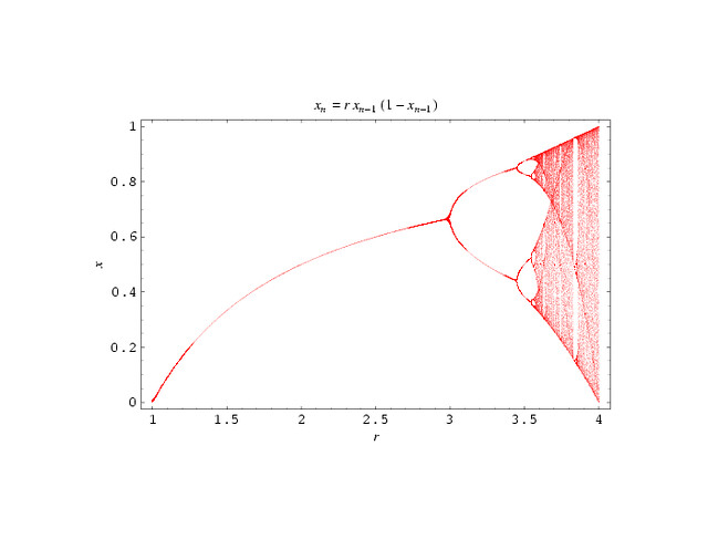
We see that as r (sometimes called the biotic potential) increases the value of the stable attractor does as well, until r reaches 3, at which point the system bifurcates. The periodic solutions grow steadily apart with increasing r, split again at r ~ 3.45, then again at ~3.54, and does this over and over again until at 3.6 the system is sampling everything in the space between about 0.3 < x < 0.9. Our stable attractor has become a strange attractor, a region (not a fixed point) of phase space to which chaotic trajectories tend, but in which behavior is nonperiodic and in which trajectories arbitrarily close to each other at one point in time will be arbitrarily far apart at another. By r = 4 the trajectories are wandering over the entirety of phase space.
What a difference discretization can make.
In fact one can get a lot more mileage out of these exercises. Here are a few more:
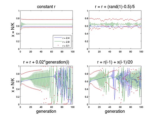
The top left is the standard plot using 3 values of r. I left off connecting the dots for the r = 3.1 case (red dots) to minimize clutter -- the 2 solutions should be evident nonetheless. The top right shows the same, only allowing r to fluctuate randomly 10% in either direction. If I had chosen a larger initial value of r or allowed larger fluctuations -- say, + / - 30% -- the system could easily have tipped into chaos. The bottom left increments r 2% per generation -- perhaps representing improvements in technology with time. Note especially the blue line: x increases smoothly and monotonically until some critical threshold is crossed and the system becomes chaotic. The bottom right has r dependent on the state of the system (including population) in the previous generation -- perhaps reflecting historical inertia and, at large x, efficiencies from economies of scale. Again the blue line is interesting, smooth growth until a threshold is crossed. The green line shows wild fluctuations until a different type of threshold is reached, whereupon there is smooth sailing for about a dozen generations before chaos once again ensues. You do not need major changes in r (bunnies developing opposable thumbs, e.g., or inventing plasma rifles) to get massive changes in x.
On steady state economies
There are any number of excellent reasons why a steady state economy is a terrible and undesireable thing, but they are beyond the scope of this post. There is only one reason why it is a good thing: in the end, the only alternative is persistent and rapid negative growth (crash and burn). By definition, a steady state economy is bounded, and treatments generally assume some indefinitely sustainable carrying capacity (a fixed attractor). But what is that value, and how could we possibly estimate it?
I do not expect either the differential or the difference form of the logistic equation to describe said carrying capacity. For one thing, I suspect that we are already in overshoot (x > 1) in some important respects. 5% of the population take up 25% of global energy consumption: if the entire world were to reach US standards of consumption we'd need to increase energy production 6-fold. It's not just a matter of quantity, rates are important as well. For another, there is no feedback term between population and environment, not explicitly anyway, and beyond a certain point, the greater the demands on the latter the greater the stresses on the former. That is, r will depend on x, and may well decrease with x at large x. And these are really just simple 1-D models of a complex and multidimensional world. Yet perhaps some of the lessons of the logistic equation are relevant all the same.
If in this one respect the system behaves more like the differential form, then higher r will only let us reach carrying capacity more quickly. If it behaves more like the difference form then higher r will allow a larger population -- up to a point, beyond which chaos might rapidly ensue. In such a case the incentive will be to keep maximizing that r until we've gone right past the maximum (and unknown) value of the fixed attractor (if such a thing is possible), which could be disastrous. Strange attractors need not (and generally do not) encompass the entire phase space, such as is the case for r = 4 in the logistic difference equation, but they may well visit enough points to cause rapid and fundamentally destabilizing changes in population or lifestyle, if in fact the system were to become chaotic. We have, it should be added, no reason to think that it will -- and no reason to think that it that it won't.
What does carrying capacity even mean? Just the term implies some maximum population that can be maintained sustainably, given some level of (fuzzily defined) health and prosperity. Is it dependent on the growth rate, or population size itself? If overshoot is possible, how would we even know what sustainability means? The problem is not simply one of population: it is also one of consumption. How do we live within our means when we do not and possibly cannot know what those means are? Some things to think about ....
